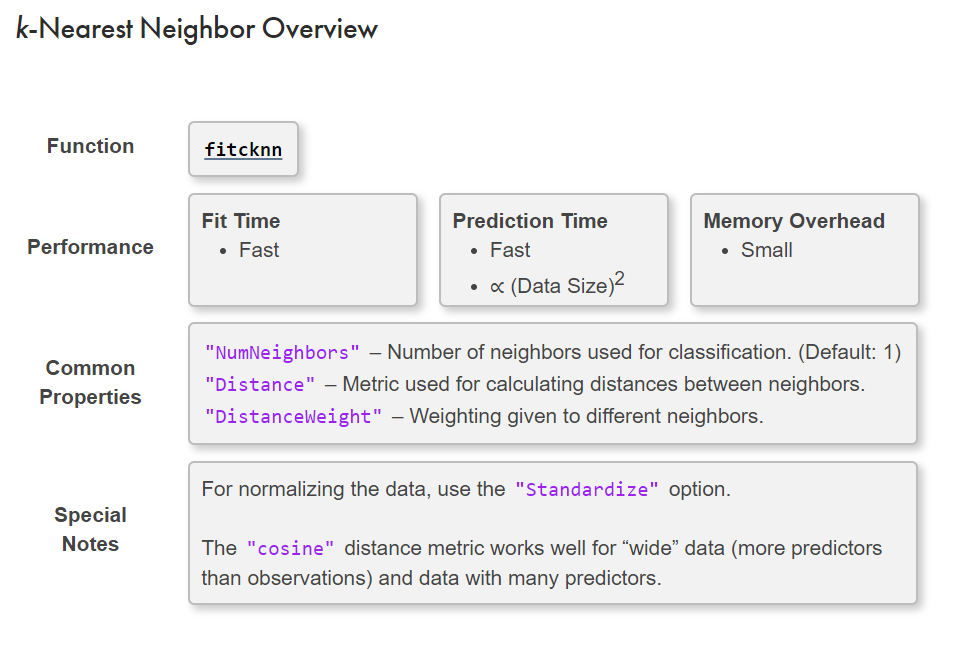
監督式學習-分類方法
KNN method
(1)Table data
如下有一表格資料 groupData (92X3)
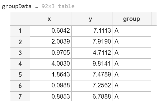
step 1: 拆成訓練資料與測試資料

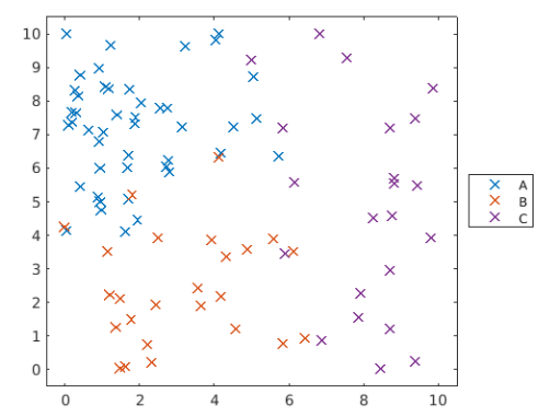
可繪製散點圖,來看訓練用資料的分群狀況
groupDataplotGroup(groupData,groupData.group,"x")
step 2: 訓練模型
Construct a k-nearest neighbor classifier named 'mdl' where k = 3. Train the model using 'dataTrain' with the response variable 'group'.
mdl = fitcknn(dataTrain,"group","NumNeighbors",3);
step 3: 測試模型
Predict the groups for the data in 'dataTest'. Assign the result to a variable named 'pg3'.
pg3 = predict(mdl,dataTest);
step 4: 可視化分類模型
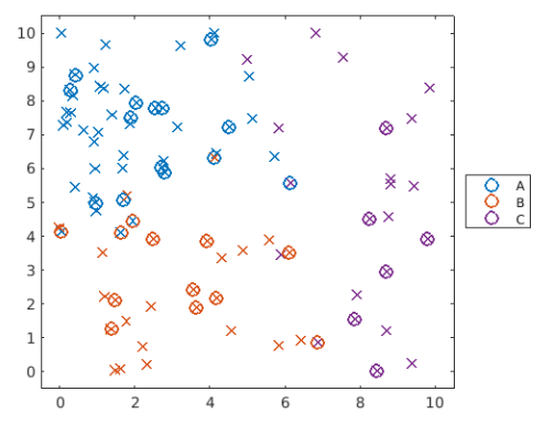
可以與step1的分類一起比較,如下
Use 'plotGroup' to plot the predicted groups for 'dataTest' with the marker "o". Use hold on and hold off to add this plot to the existing figure.
hold on
plotGroup(dataTest,pg3,"o")
hold off
step 5: 驗證模型
一種確認模型是否能正確分類的方法是,採用 loss 函數,即誤報率。
Notice the point near (7,1) which has been misclassified. The true class (x marker) is different from the predicted class (o marker). What proportion of points have been misclassified?
Calculate the loss for the test data 'dataTest', and assign it to a variable named 'err3'.
err3 = loss(mdl,dataTest)
step 6: 修改模型
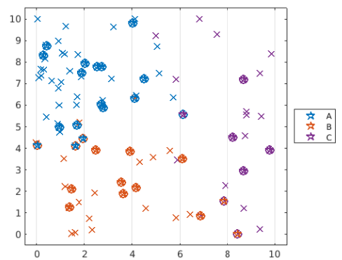
可以試著調整 nearest neighbors 來改善模型
mdl.NumNeighbors = 10;
step 7: 重新測試與可視化模型
pg10 = predict(mdl,dataTest);
hold on
plotGroup(dataTest,pg10,"p")
hold off
(2)Array data
與 table 資料類似,但現在改成陣列來處理
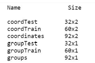
step 1: 拆成訓練資料與測試資料
step 2: 訓練模型
mdl = fitcknn(coordTrain,groupTrain,"NumNeighbors",3);
step3 : 測試模型
predGroups = predict(mdl,coordTest);
step4: 驗證模型
mdlLoss = loss(mdl,coordTest,groupTest)
Decision Trees
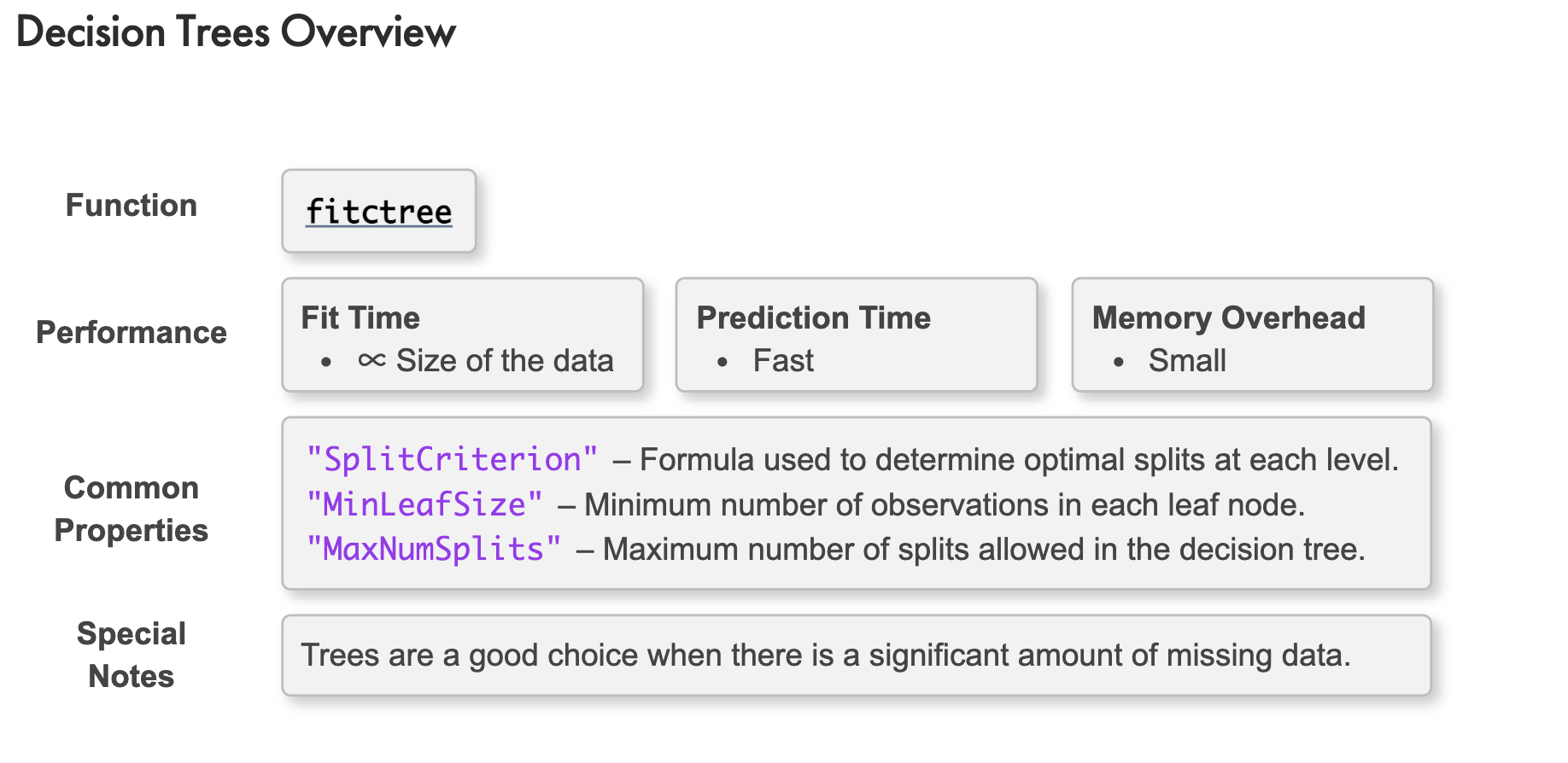
下表列出一組心臟病資料:
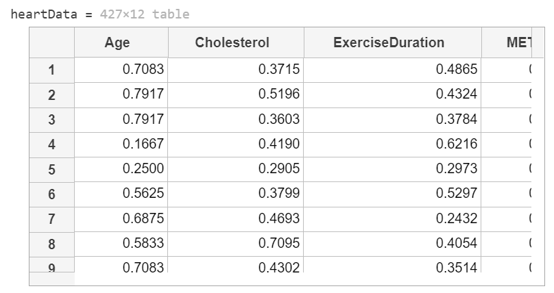
This code loads and formats the data.
heartData = readtable("heartDataNum.txt");
heartData.HeartDisease = categorical(heartData.HeartDisease);
This code partitions the data into training and test sets.
pt = cvpartition(heartData.HeartDisease,"HoldOut",0.3);
hdTrain = heartData(training(pt),:);
hdTest = heartData(test(pt),:);
Create a classification tree model named mdl using the training data 'hdTrain'
mdl = fitctree(hdTrain,"HeartDisease");
Change the level of branching of mdl to 3.
mdl = prune(mdl,"Level",3)
最後驗證模型
errTrain = resubLoss(mdl);
errTest = loss(mdl,hdTest);
disp("Training Error: " + errTrain)
disp("Test Error: " + errTest)
Naïve Bayes
決策樹與KNN分類法都沒有對資料進行假設,但‘單純貝氏分類’是一系列以假設特徵之間強(樸素)獨立下運用貝葉斯定理為基礎的簡單機率分類器
If we assume the data set comes from an underlying distribution, we can treat the data as a statistical sample. This can reduce the influence of the outliers on our model.
A naïve Bayes classifier assumes the independence of the predictors within each class. This classifier is a good choice for relatively simple problems.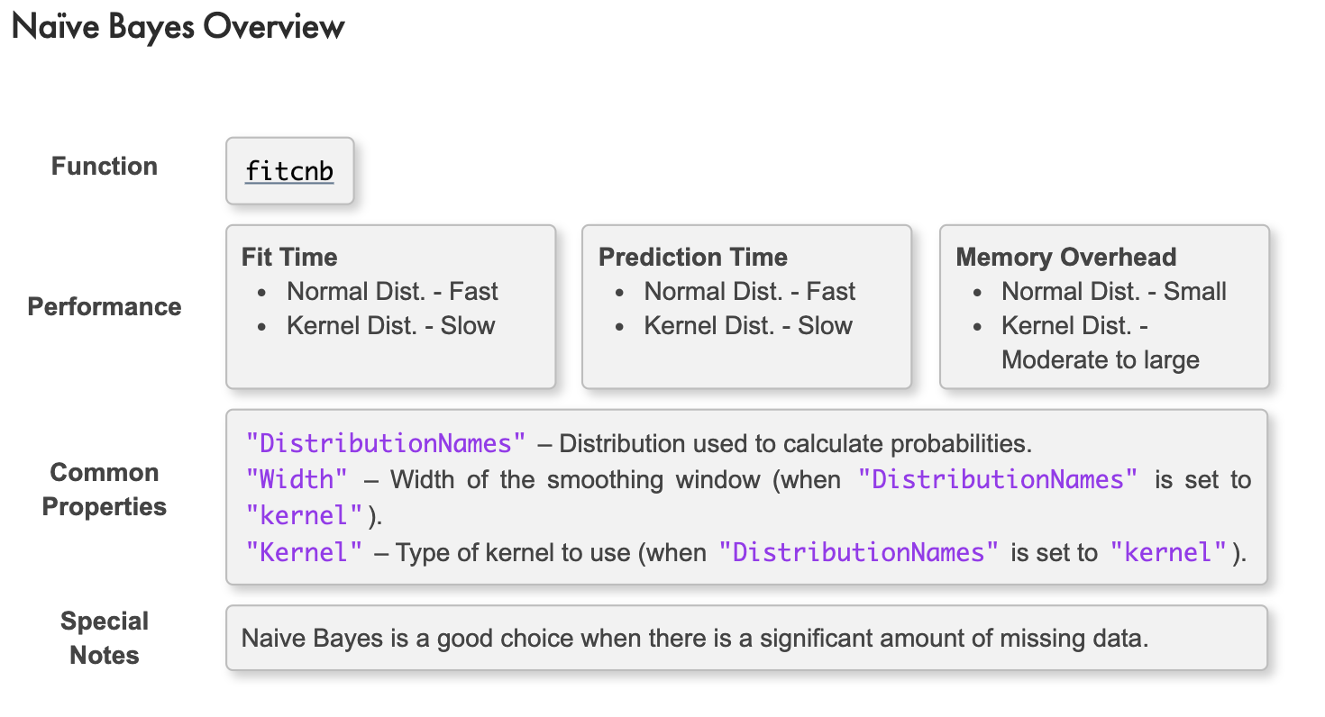
Discriminant Analysis
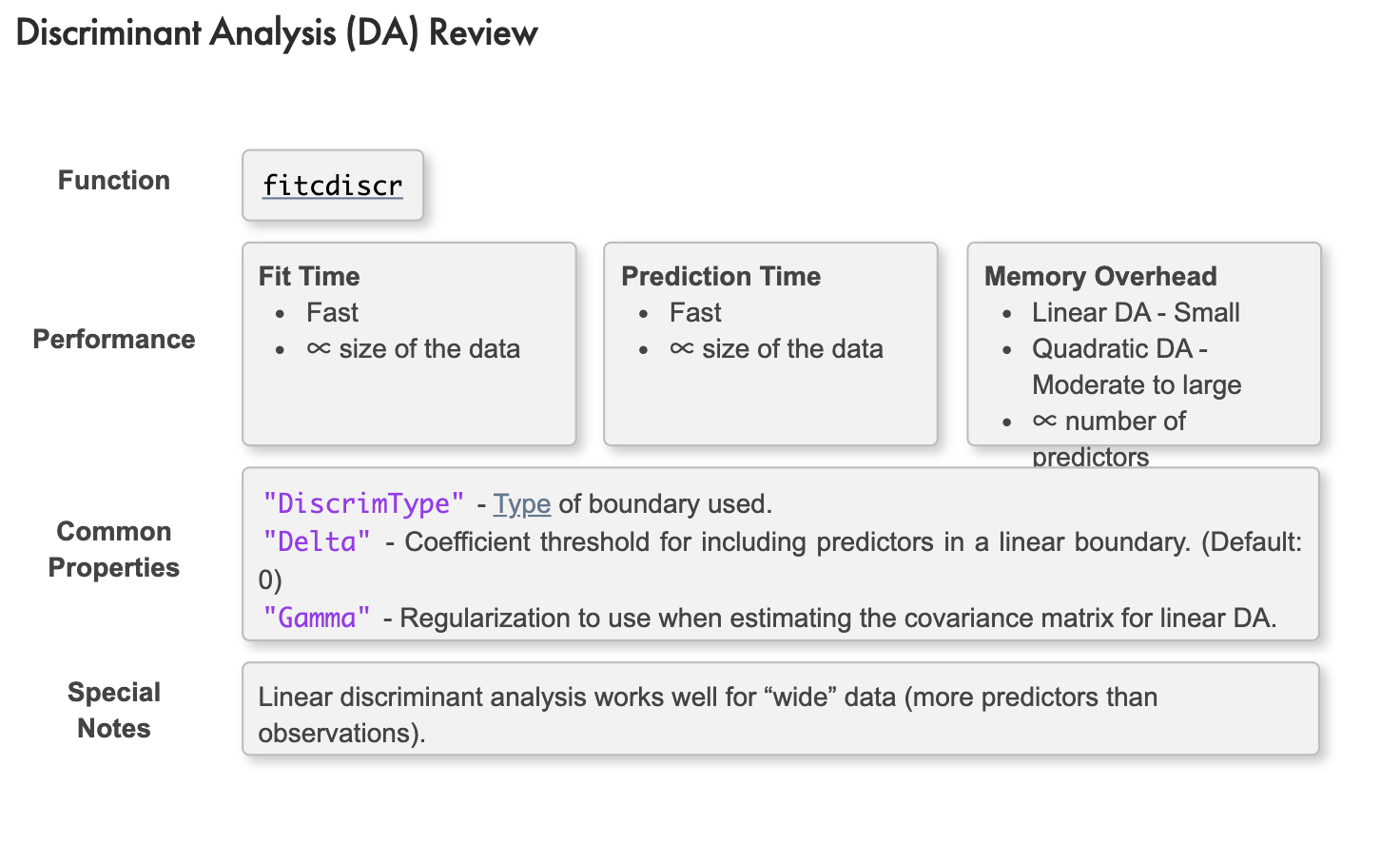
判別分析,又稱為線性判別分析(Linear Discriminant Analysis),是利用已知類別的樣本建立判別模型,為未知類別的樣本判別的一種統計方法。
Similar to naive Bayes, discriminant analysis works by assuming that the observations in each prediction class can be modeled with a normal probability distribution. However, there is no assumption of independence in each predictor. Hence, a multivariate normal distribution is fitted to each class.
Linear Discriminant Analysis
By default, the covariance for each response class is assumed to be the same. This results in linear boundaries between classes.
daModel = fitcdiscr(dataTrain,"ResponseVarName")
Quadratic Discriminant Analysis
Removing the assumption of equal covariances results in a quadratic boundary between classes. Use the "DiscrimType" option to do this:
daModel = fitcdiscr(dataTrain,"ResponseVarName","DiscrimType","quadratic")
Support Vector Machines
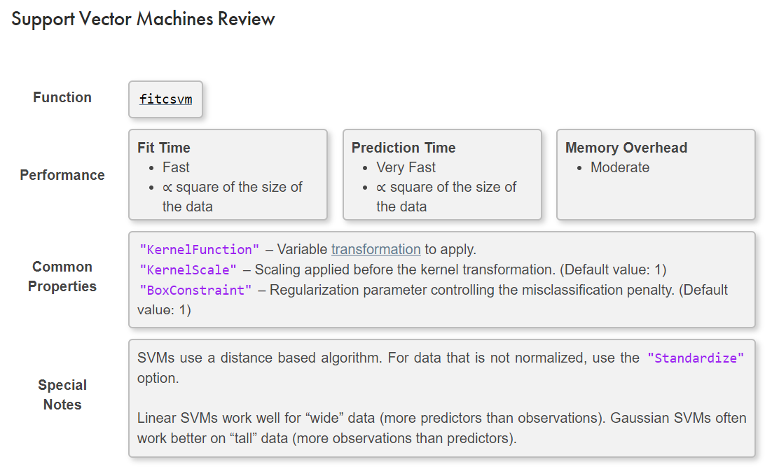
A Support Vector Machine (SVM) algorithm classifies data by finding the "best" hyperplane that separates all data points.

Step1: process data
如下程式碼,已經將一組透過cvpartition 將資料分類
load groups
cvpt = cvpartition(groupData.group,"Holdout",0.35);
dataTrain = groupData(training(cvpt),:);
dataTest = groupData(test(cvpt),:);
Step2: 訓練模式與驗證
mdlSVM = fitcsvm(dataTrain,"group","KernelFunction","gaussian");
errSVM = loss(mdlSVM,dataTest)
Step3: 可視化資料
predGroups = predict(mdlSVM,dataTest);
plotGroup(groupData,groupData.group,"x")
hold on
plotGroup(dataTest,predGroups,"o")
hold off
其中,function plotGroup 如下:
function plotGroup(data,grp,mkr)
validateattributes(data,"table",{'nonempty','ncols',3})
% Plot data by group
colors = colororder;
p = gscatter(data.x,data.y,grp,colors([1 2 4],:),mkr,9);
% Format plot
[p.LineWidth] = deal(1.5);
legend("Location","eastoutside")
xlim([-0.5 10.5])
ylim([-0.5 10.5])
end
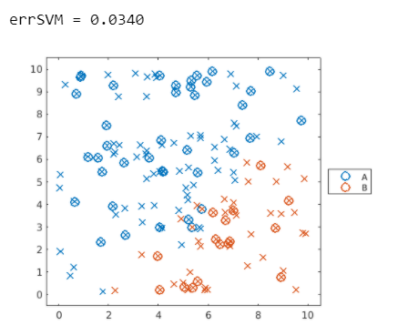
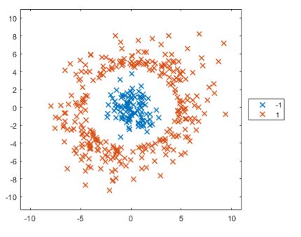
上圖可以發現,仍有一些資料沒有分類正確,下例中測試另一種數據,稱為同心圓數據。
Step1: process data
load points
rng(123)
cvpt = cvpartition(points.group,"Holdout",0.38);
trainPoints = points(training(cvpt),:);
testPoints = points(test(cvpt),:);
plotGroup(points,points.group,"x")
Step2: 訓練模式與驗證繪圖
mdl = fitcsvm(trainPoints,"group","KernelFunction","polynomial");
mdlLoss = loss(mdl,testPoints)
predGroups = predict(mdl,testPoints);
plotGroup(points,points.group,"x")
hold on
plotGroup(testPoints,predGroups,"o")
hold off
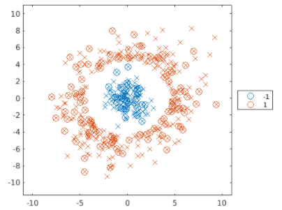
換言之,SVM適合分類非線性的資料
Multiclass Support Vector Machine Models
perform multiclass SVM classification by creating an error-correcting output codes (ECOC) classifier.
例如下圖應該有三個類別的數據
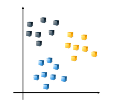
Suppose there are three classes in the data. By default, the ECOC model reduces the model to multiple, binary classifiers using the one-vs-one design.
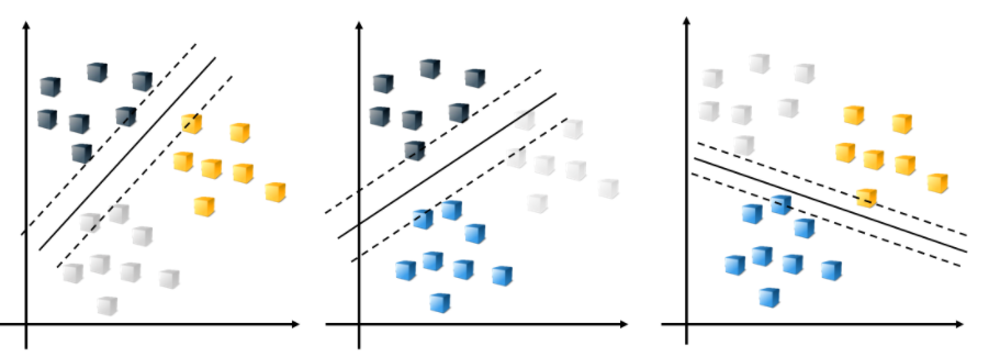
The combination of the resulting classifiers is used for prediction.

Creating a multiclass SVM model is a two-step process.
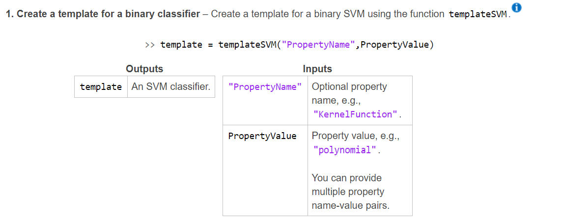
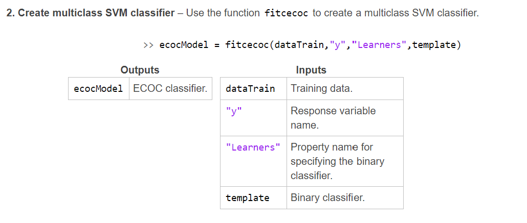
如˙下一組資料,欲進行Multiclass Support Vector Machine Models
load groups
rng(0)
cvpt = cvpartition(groupData.group,"Holdout",0.35);
dataTrain = groupData(training(cvpt),:);
dataTest = groupData(test(cvpt),:);
plotGroup(groupData,groupData.group,"x")
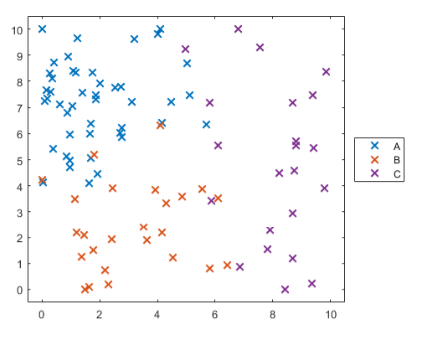
Create a multiclass SVM classifier named 'mdlMSVM' using the training data 'dataTrain' and the response variable 'group'. Calculate the classification loss for the test data 'dataTest', and name it 'errMSVM'.
mdlMSVM = fitcecoc(dataTrain,"group");
errMSVM = loss(mdlMSVM,dataTest)
predGroups = predict(mdlMSVM,dataTest);
plotGroup(groupData,groupData.group,"x")
hold on
plotGroup(dataTest,predGroups,"o")
hold off
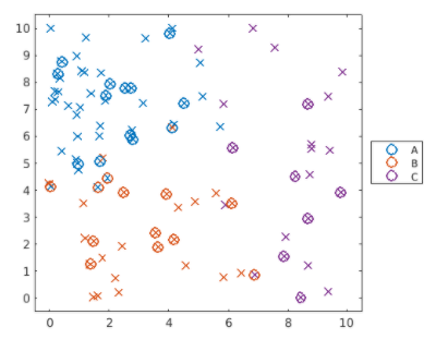
上圖的分類並不成功,loss大約0.1588,create a template learner by passing the property name-value pairs to the ‘templateSVM’ function.
t = templateSVM("PropertyName",PropertyValue);
Then provide the template learner to the ‘fitcecoc’ function as the value for the Learners property.
mdl = fitcecoc(tableData,"Response", "Learners",t);
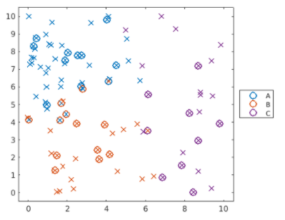
如下程式碼,針對上圖做修改
Create 'mdlMSVM' so that it uses the value "polynomial" for the "KernelFunction" property. Calculate the loss errMSVM for the new model.
template = templateSVM("KernelFunction","polynomial");
mdlMSVM = fitcecoc(dataTrain,"group","Learners",template);
errMSVM = loss(mdlMSVM,dataTest)
實務範例
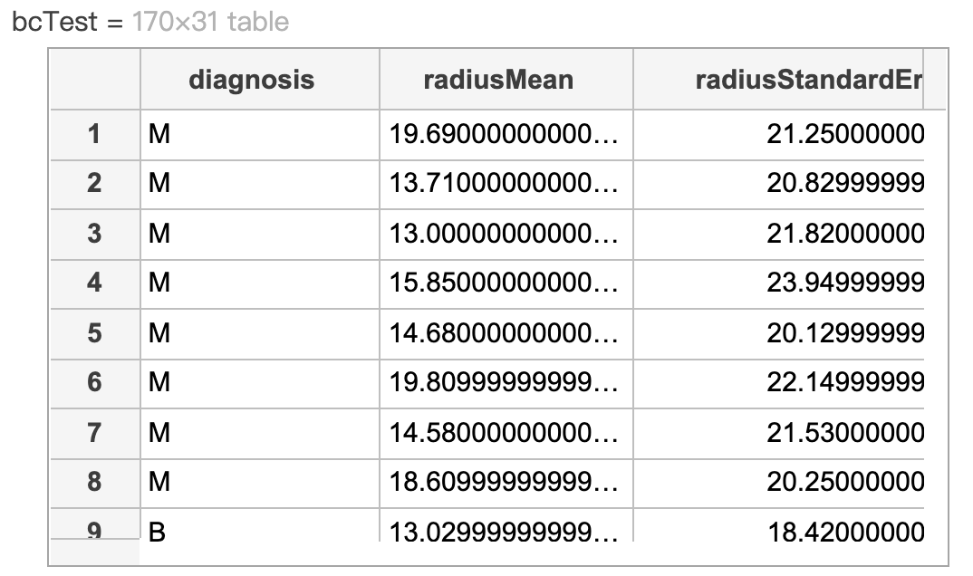
下表為一組乳腺癌圖像數字化的資料, "diagnosis" 為 response variable
step 1: 讀取與分割資料
bcDiag = readtable("breastCancerData.txt");
bcDiag.diagnosis = categorical(bcDiag.diagnosis);
pt = cvpartition(bcDiag.diagnosis,"HoldOut",0.3);
bcTrain = bcDiag(training(pt),:);
bcTest = bcDiag(test(pt),:)
step 2: 訓練模型與計算misclassification loss
mdl = fitcknn(bcTrain,"diagnosis","NumNeighbors",5);
errRate = loss(mdl,bcTest)
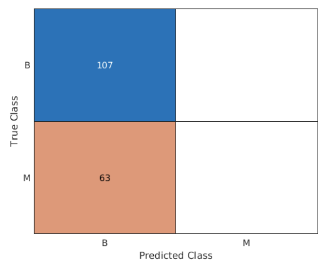
step 3: 計算假陰性與繪製confustion chart
False negatives (假陰性) 代表診斷是惡性但預測為良性
p = predict(mdl,bcTest);
falseNeg = mean((bcTest.diagnosis == "M") & (p == "B"))
confusionchart(bcTest.diagnosis,p);
