Linear Regression Models
Linear regression is one of the simplest but most powerful-regression techniques. It is a parametric regression technique in which the response is modeled as some known formula given in terms of the predictor variables.
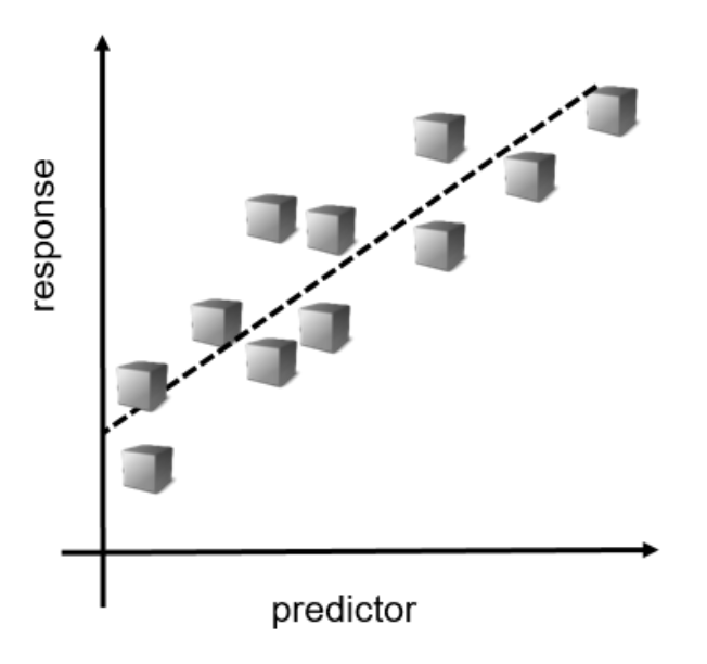
Use the function fitlm to fit a linear regression model.
mdl = fitlm(data,"modelspec")

The first input to fitlm is a table containing the predictors and the response. By default, fitlm uses the last column as the response and all other columns as predictors.
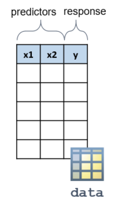
When modeling a linear regression, you can apply different functions to the predictive variables.
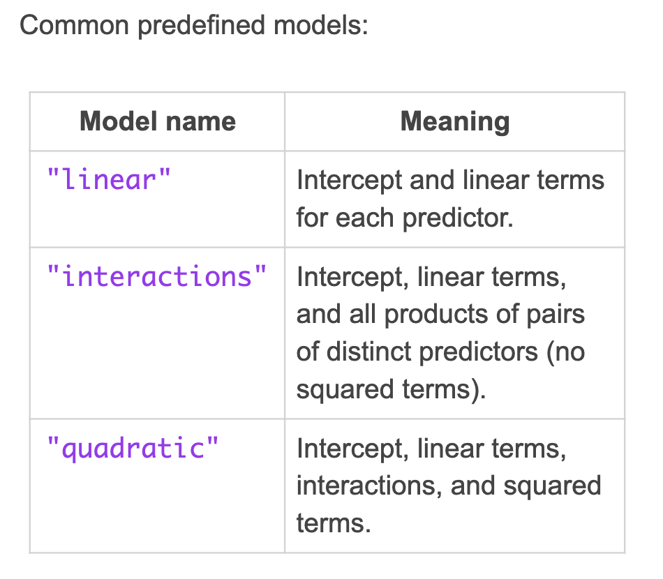
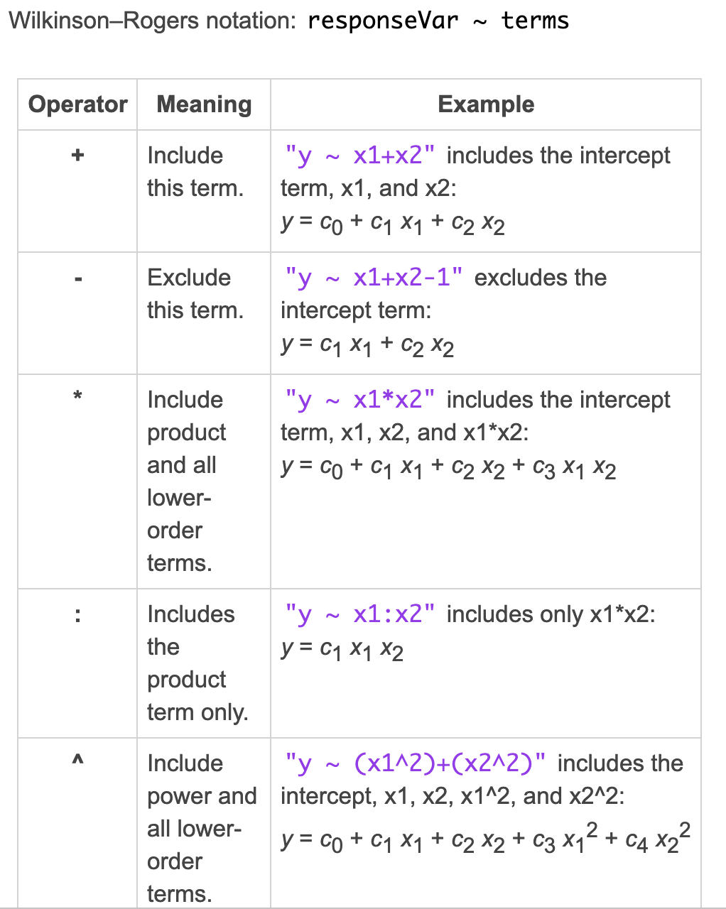
As the second input to fitlm, you can use one of the predefined models or you can specify a model by providing a formula in Wilkinson-Rogers notation.
Fitting a Line
如下表範例
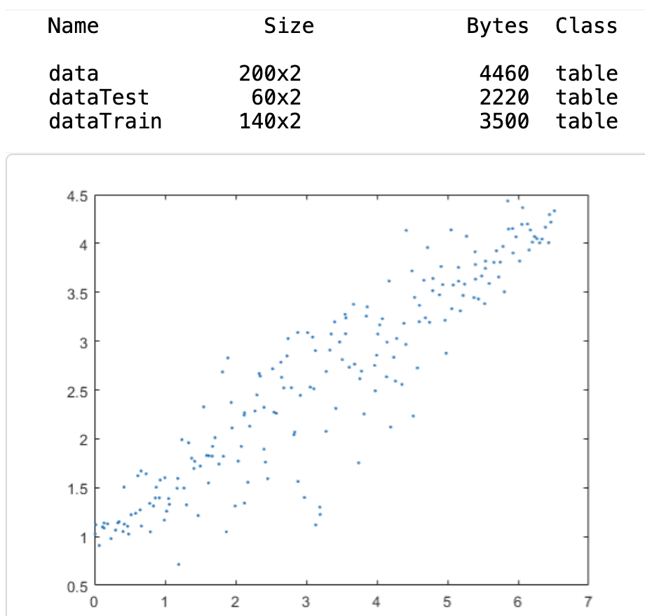
load data
whos data dataTrain dataTest
plot(data.x,data.y,".")
(1) training model
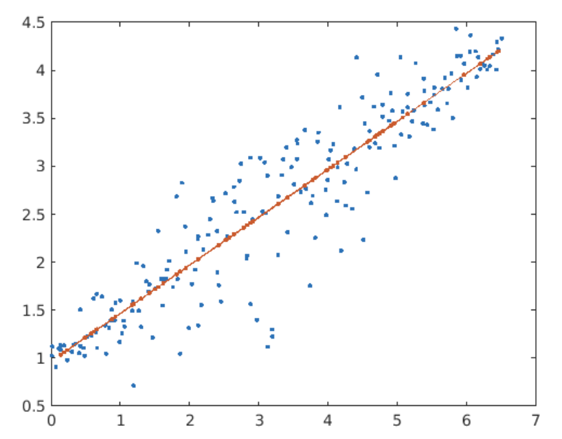
mdl = fitlm(dataTrain)
(2) prediction
Pred = predict(mdl, dataTest)
(3) plot figure
hold on
plot(dataTest.x,yPred,".-")
hold off
Fitting a Polynomial
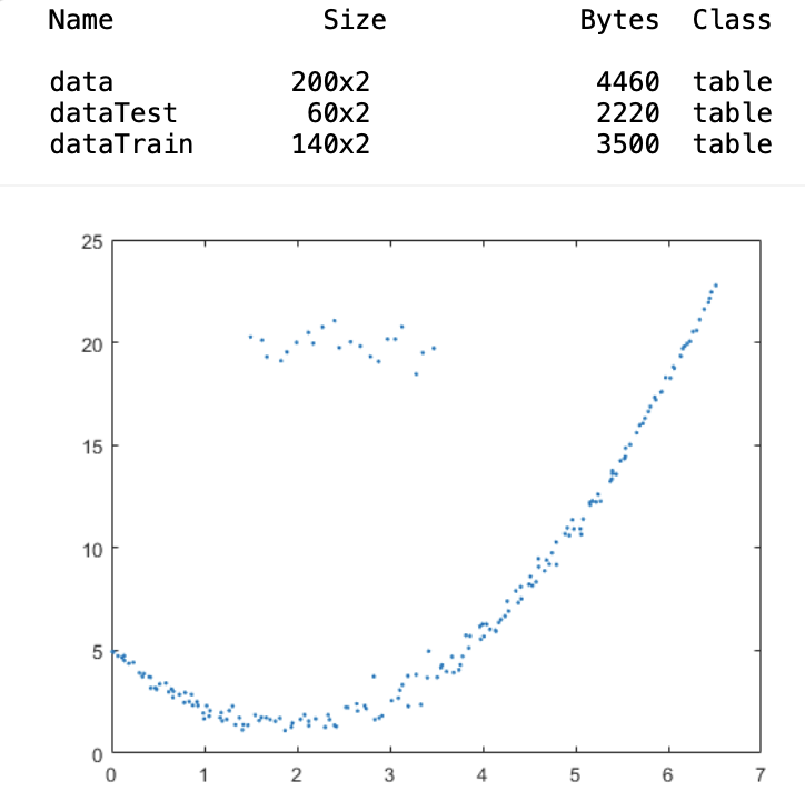
使用資料如下圖
(1) fits a quadratic polynomial to the training data.
mdl = fitlm(dataTrain,"quadratic")
yPred = predict(mdl,dataTest);
(2) plot
plot(data.x,data.y,".")
hold on
plot(dataTest.x,yPred,".")
hold off
legend("All Data","Predicted Response")
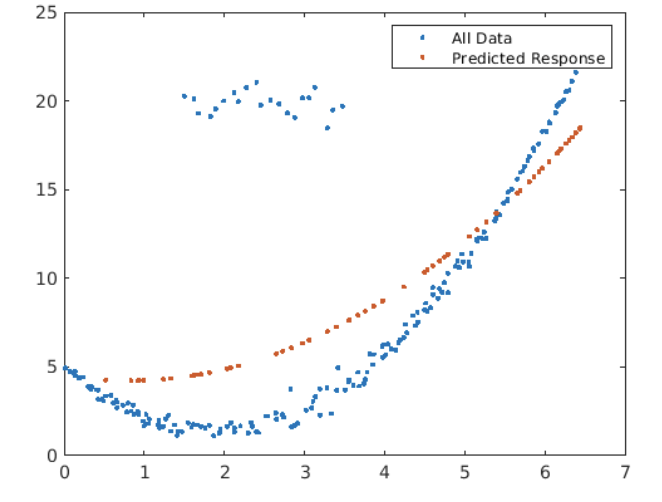
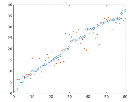
Notice the cluster of outliers in the upper left of the plot.
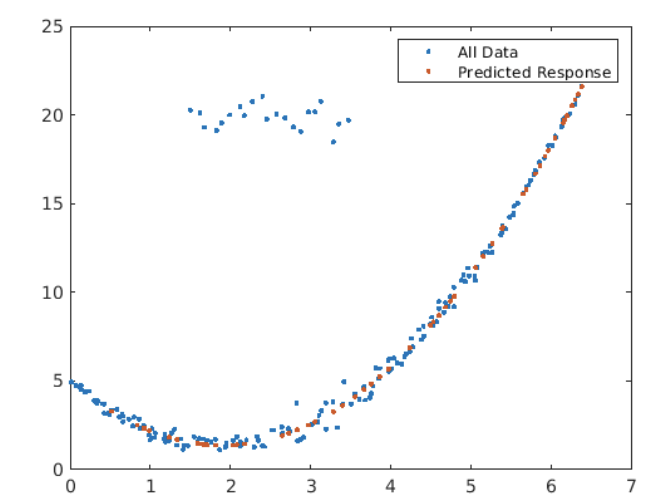
You can reduce the influence of the outliers on the model by setting the "RobustOpts" property to "on".
mdl = fitlm(dataTrain,"quadratic","RobustOpts","on")
yPred = predict(mdl,dataTest);
Multivariable Linear Regression
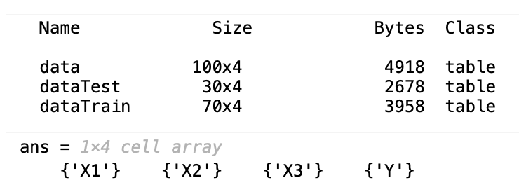
The table data has three predictor variables (X1, X2, X3) and one response (Y). It has been split into training and test sets: dataTrain and dataTest.
You can find a reference for Wilkinson-Rogers notation in the documentation.
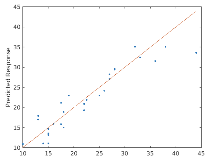
Modify your code so that mdl fits a model where the response Y is a function of X1, X1^2, and X3.
mdl = fitlm(dataTrain,"Y ~ X3 + X1^2")
yPred = predict(mdl,dataTest);
Fitting Models Using Data Stored in Arrays
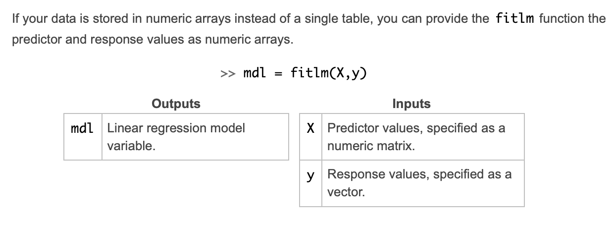
Each column of the predictor matrix X is treated as one predictor variable. By default, fitlm will fit a model with an intercept and a linear term for each predictor (column).
To fit a different regression formula, you have two options.
You can store the predictors and the response in a table and provide the model specification separately.
Alternatively, you can create a matrix with a column for each term in the regression formula. This matrix is called a design matrix.
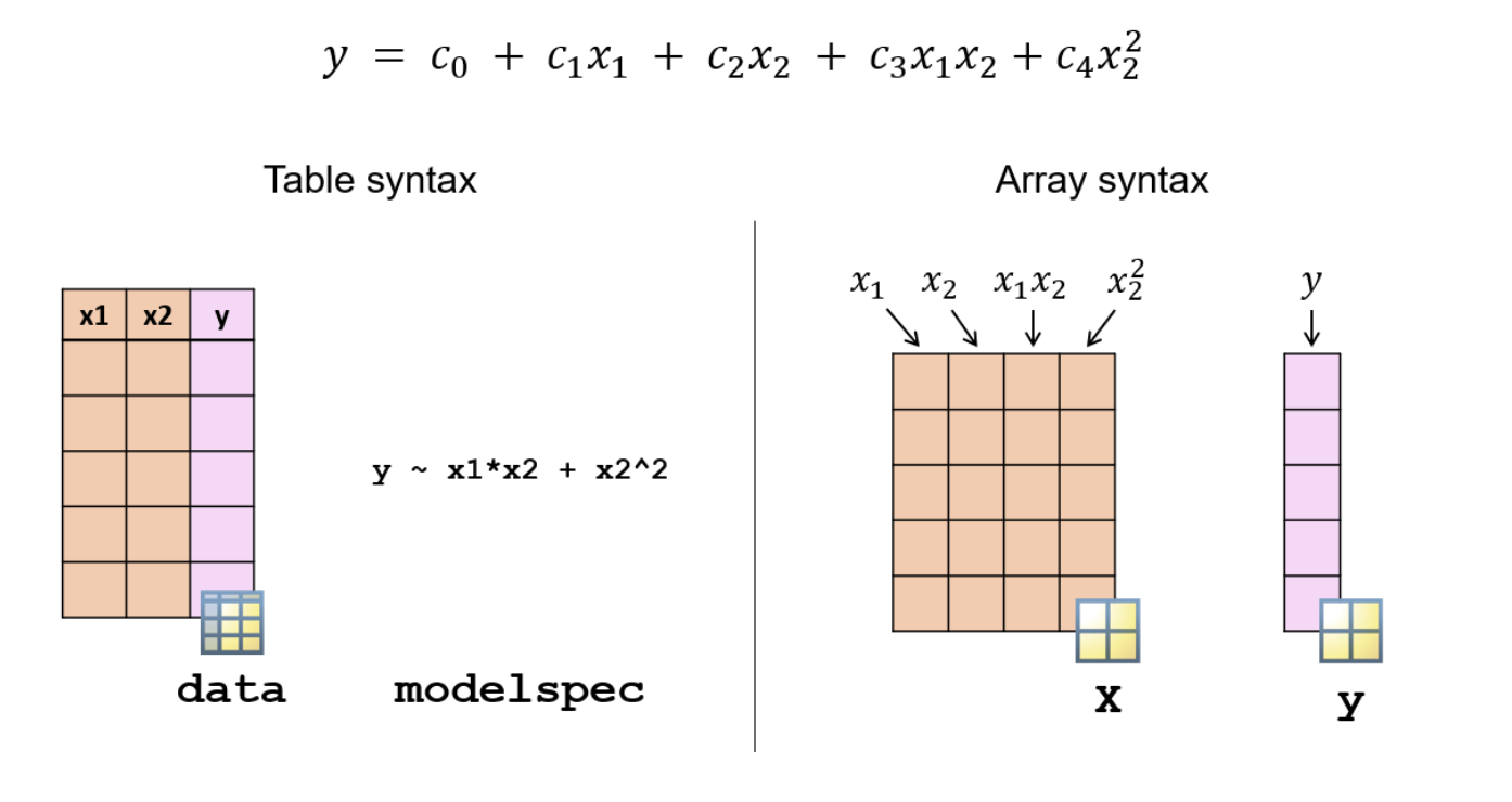
如下範例
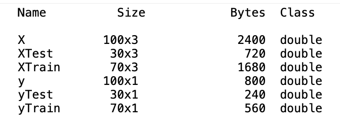
Create a regression model named 'mdl' fitting the training data. Use a linear combination of the predictor variables for the model.
mdl = fitlm(XTrain,yTrain)
When you provide training data to fitlm as a numeric array, each column represents a term in the regression formula. This matrix is the design matrix.
for example:
XTrain13 = [XTrain(:,1),XTrain(:,3),XTrain(:,1).*XTrain(:,3)];
mdl13 = fitlm(XTrain13,yTrain)
Stepwise Linear Regression
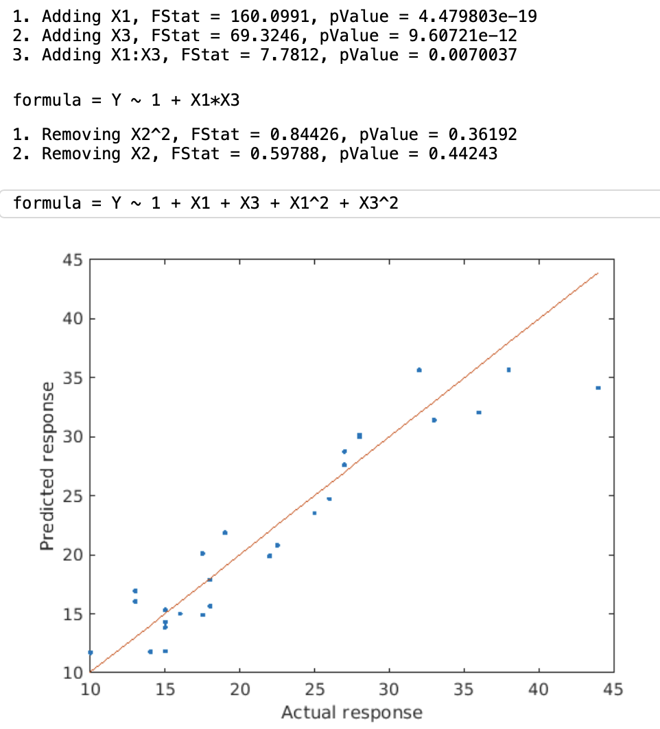
Stepwise linear regression methods choose a subset of the predictor variables and their polynomial functions to create a compact model.
Note The stepwiselm function is used only when the underlying model is linear regression. For nonlinear regression and classification problems, use the function sequentialfs.
Use the function stepwiselm to fit a stepwise linear regression model.
stepwiseMdl = stepwiselm(data,"modelspec")

stepwiselm chooses the model for you. However, you can provide the following inputs to control the model selection process.
- "modelspec" - The second input to the function specifies the starting model. stepwiselm starts with this model and adds or removes terms based on certain criteria.
Commonly used starting values: "constant", "linear", "interactions" (constant, linear, and interaction terms), "quadratic" (constant, linear, interaction, and quadratic terms). - "Lower" and "Upper" - If you want to limit the complexity of the model, use these properties. For example, the following model will definitely contain the intercept and the linear terms but will not contain any terms with a degree of three or more.
mdl = stepwiselm(data,"Lower","linear","Upper","quadratic")
- By default, stepwiselm considers models as simple as a constant term only and as complex as an interaction model.
for example
mdl = stepwiselm(dataTrain);
yPred = predict(mdl,dataTest);
formula = mdl.Formula
or
yPred = predict(mdl,dataTest);
formula = mdl.Formula
Regularized Linear Regression
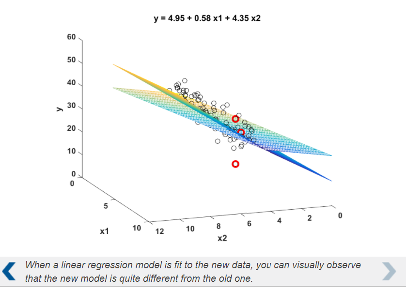
When a data set has a large number of predictors, choosing the right parametric regression model can be a challenge. Including all the predictors can create an unnecessarily complicated model, and some of the predictors can be correlated.
Regularization
Regularized linear regression models shrink the regression coefficients by applying a penalty for large coefficient values. This reduces the variance of the coefficients and can create models with smaller prediction error.

Ridge and Lasso Regression
In linear regression, the coefficients are chosen by minimizing the mean squared error (MSE). Mean squared error is the squared difference between the observed and the predicted response value.
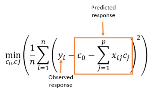
In ridge and lasso regression, a penalty term is added to MSE.

- Ridge regression shrinks coefficients continuously, and keeps all predictors.
- Lasso allows coefficients to be set to zero, reducing the number of predictors included in the model.
Lasso can be used as a form of feature selection, however feature selection may not be appropriate for cases with similar, highly correlated variables. It may result in loss of information which could impact accuracy and the interpretation of results. Ridge regression maintains all features, but the model may still be very complex if there is a large number of predictors.
Fitting Ridge Regression Models
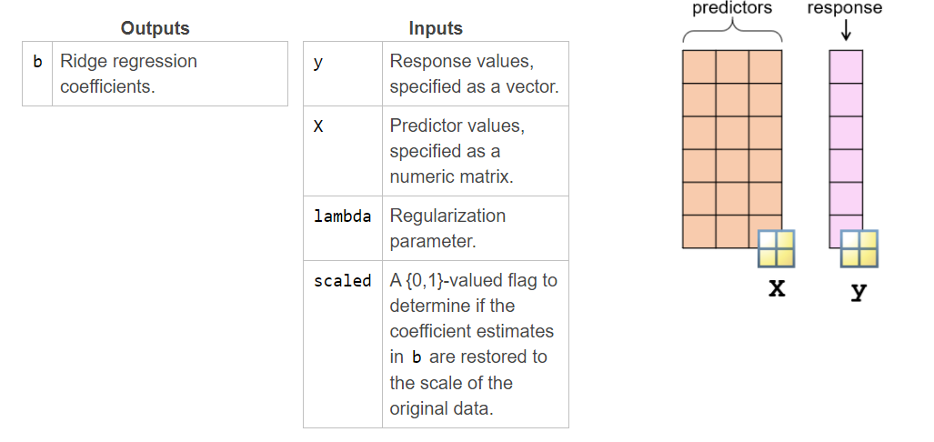
You can use the function ridge to fit a ridge regression model.
b = ridge(y,X,lambda,scaled)
Determining the Regression Parameter
When you provide a vector of λ values to the ridge function, the output b is a matrix of coefficients.
The columns of b contain the coefficient values for each parameter in the vector lambda.
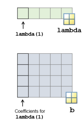
You can now use each column of the matrix b as regression coefficients and predict the response.
yPred = dataNew*b(2:end,:) + b(1,:);
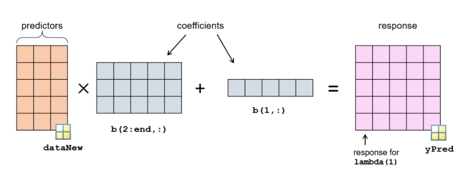
The response yPred is a matrix where each column is the predicted response for the corresponding value of lambda. You can use yPred to calculate the mean squared error (MSE), and choose the coefficients which minimize MSE.
Fitting a Ridge Regression Model
如下範例
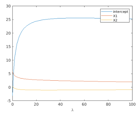
lambda = 0:100;
b = ridge(yTrain,XTrain,lambda,0);
plot(lambda,b)
legend("intercept","X1","X2")
xlabel("\lambda")
yPred = b(1,:) + XTest*b(2:end,:);
err = yPred - yTest;
mdlMSE = mean(err.^2);
plot(lambda,mdlMSE)
xlabel("\lambda")
ylabel("MSE")
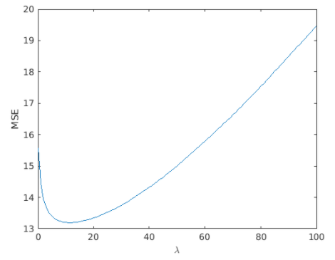
[minMSE,idx] = min(mdlMSE)
plot(yTest,"o")
hold on
plot(yPred(:,idx),".")
hold off
