Machine learning problems often involve high-dimensional data with hundreds or thousands of predictors. For example:

• Facial recognition problems can involve images with thousands of pixels and each pixel can be treated as a predictor.


• Predicting weather can involve analyzing temperature and humidity measurements at thousands of locations.

Feature transformation 

Transform the coordinate space of the observed variables.

Principal component analysis (PCA) transforms an n-dimensional feature space into a new n-dimensional space of orthogonal components. The components are ordered by the variation explained in the data.

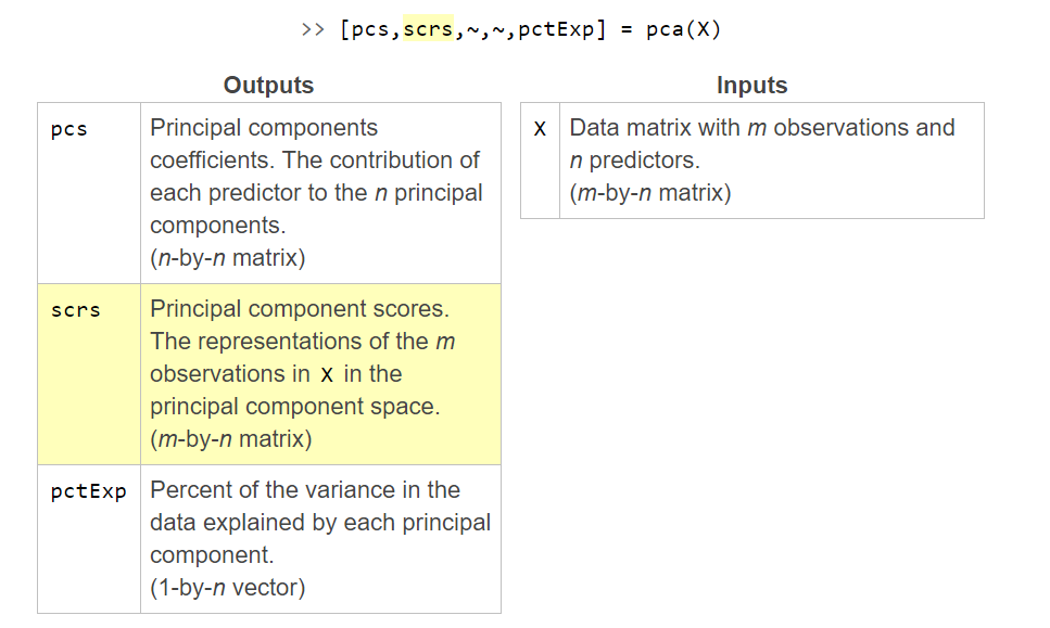
Interpreting Principal Components

The principal components by themselves have no physical meaning. However, the coefficients of the linear transformation indicate the contribution of each variable in the principal component. 

For example, if the coefficients of the first principal component are 0.8, 0.05, and 0.3, the first variable has the largest contribution followed by the third and the second variable.

Biplot

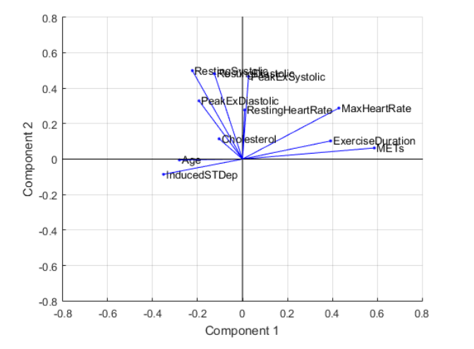
You can visualize any two principal components using the function biplot. It's commonly used to visualize the first two principal components, which explain the greatest amount of variance in the data.

biplot(pcs(:,1:2),"VarLabels",varnames) 

Heat Map

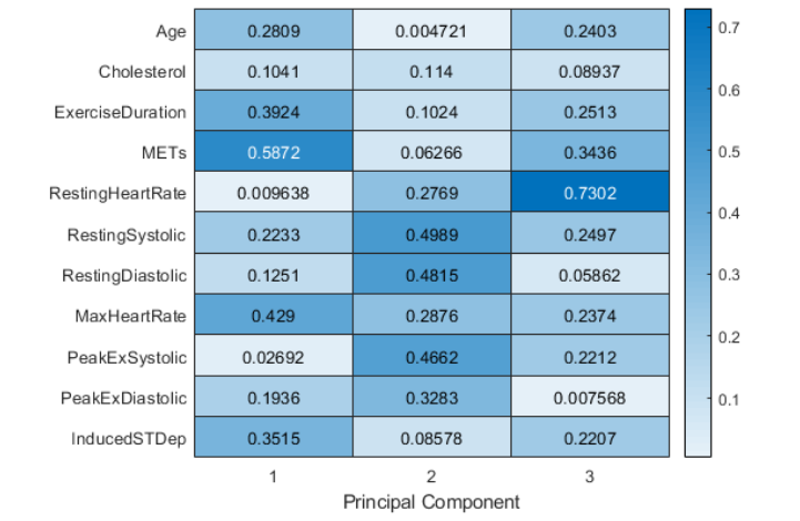
You can also visualize the contributions of each variable to the principal components as a heat map. 

heatmap(abs(pcs(:,1:3)),"YDisplayLabels",varnames); 

 xlabel("Principal Component") 

Parallel Coordinates Plot

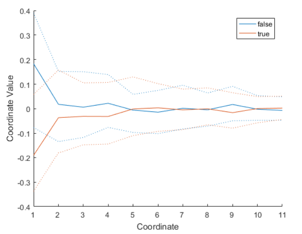
PCA can be performed independent of the response variable. However, when the data has a response variable that has multiple categories (for example, true and false), a parallel coordinates plot of the principal component scores can be useful.

parallelcoords(scrs,"Group",y,"Quantile",0.25) 

Feature selection 

Choose a subset of the observed variables.

Some classifiers have their own built-in methods of feature selection.

Decision Trees: Predictor Importance

You can use predictorImportance on a decision tree model to calculate the importance of each predictor variable.

predImp = predictorImportance(treeModel)

Note:  You cannot use the predictorImportance function with cross-validated decision tree models.

下例中示範如何運用predictorImportance函數來簡化預測變量。假設一組資料如下：

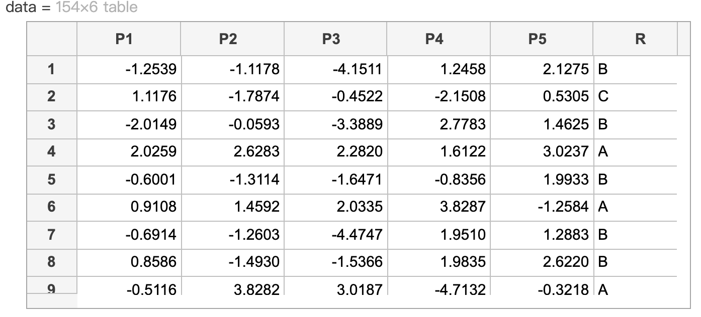
This code fits a 7-fold cross-validated classification tree model to the original data and calculates the loss.

mdlFull = fitctree(data,"R","KFold",7);

fullLoss = kfoldLoss(mdlFull)

其結果：fullLoss = 0.0844

Create a classification tree model named mdl without cross-validation. Then calculate the importance of each predictor and store the result in p.

mdl = fitctree(data,"R");

p = predictorImportance(mdl)

並繪製長條圖

bar(p)

xticklabels(data.Properties.VariableNames(1:end-1))

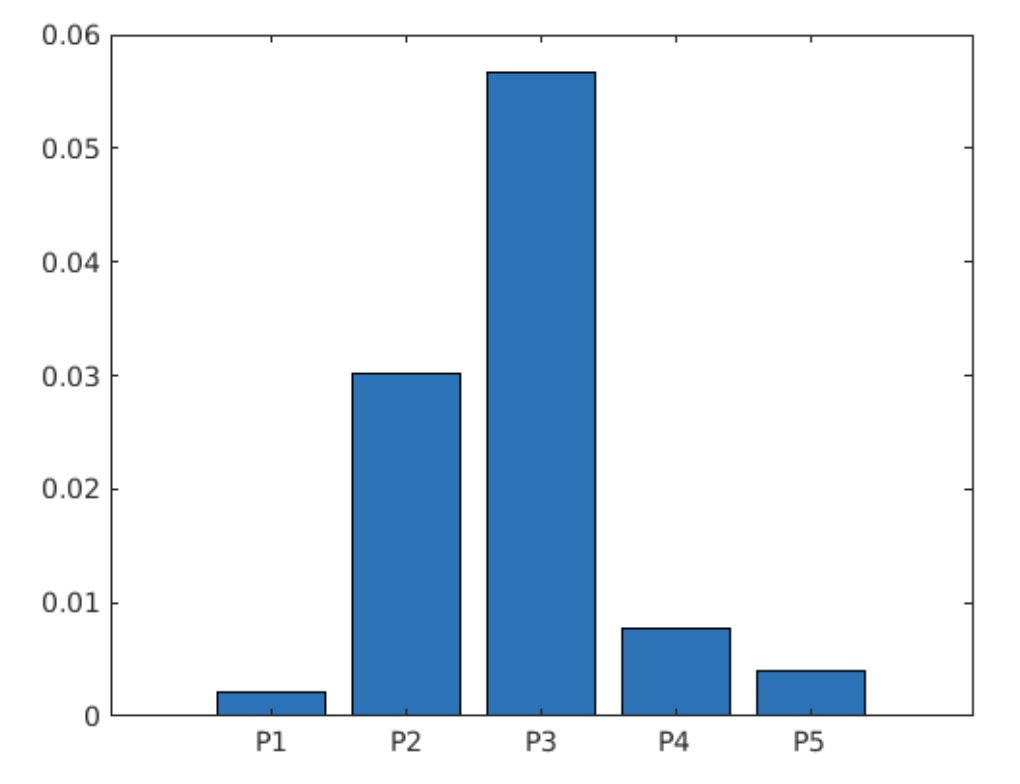
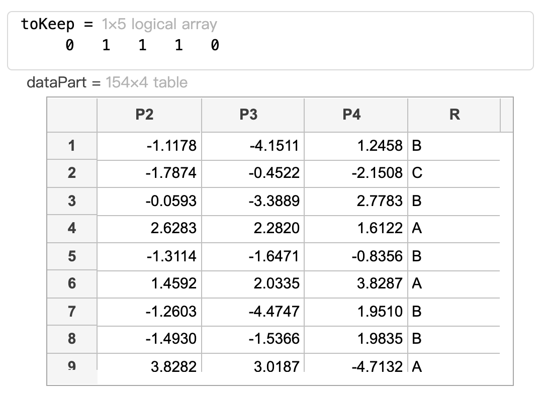
Create a logical vector ‘toKeep' whose values are true if the corresponding values of 'p' are greater than 0.005 and false otherwise. 

Use 'toKeep' to create a table 'dataPart' which contains only the predictors with 'p' greater than 0.005 and the response 'R'.

toKeep = p > 0.005

dataPart = data(:,[toKeep true])

Create a seven-fold cross-validated classification tree model named 'mdlPart' which uses only the selected predictors. Calculate the loss and save it to 'partLoss'.

mdlPart = fitctree(dataPart,"R","KFold",7);

partLoss = kfoldLoss(mdlPart)

其結果：fullLoss = 0.0909

Sequential Feature Selection

Sequential feature selection is an iterative procedure that, given a specific predictive model, adds and removes predictor variables in turn, and then evaluates the effect on the quality of the model.

The function sequentialfs performs sequential feature selection.

toKeep = sequentialfs(fun,X,y)

Note that the first input is a handle to the error function.

tokeep = sequentialfs(@errorFun,X,y)

You can use the optional property "cv" to specify the cross validation method. For example, you can specify a 7-fold cross validation.

tokeep = sequentialfs(@errorFun,X,y,"cv",7)

Sequential feature selection requires an error function that builds a model and calculates the prediction error. The error function must have the following structure.

• Four numeric inputs:
  • two for training the model (predictor matrix and response vector)
  • two for evaluating the model (predictor matrix and response vector)
• One scalar output representing the prediction error.

Note:  You do not need to create the training and test data sets. The sequentialfs function will internally partition the data before calling the error function.

An alternative to writing the error function in a local function or separate file is to create an anonymous function.

To create an anonymous function that calculates the number of misclassifications given training and test data, use the following pattern:

selected = sequentialfs(anonfun,...
predictors,response)

如下範例

（1）Create an anonymous function 並使用KNN

ferror = @(XTrain,yTrain,XTest,yTest)...

nnz(yTest ~= predict(...

fitcknn(XTrain,yTrain),XTest))

(2) 結合anonymous function，並使用邏輯向量挑選重要的預測因子

toKeep = sequentialfs(ferror,data{:,1:end-1},data.R)

dataPart = data(:,[toKeep true])

(3) 再預測一次

mdlPart = fitcknn(dataPart,"R","KFold",7);

partLoss = kfoldLoss(mdlPart)

Accommodating Categorical Data

Some algorithms and functionality (e.g., sequentialfs) requires predictors in the form of a numeric matrix. If your data contains categorical predictors, how can you include these predictors in the model?

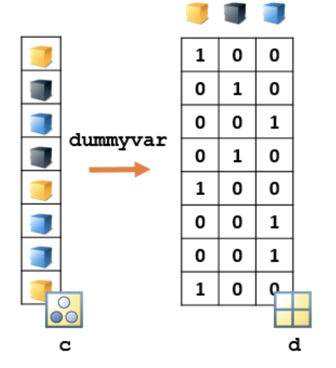
A better approach is to create new dummy predictors, with one dummy predictor for each category.

d = dummyvar(c)

Each column of d represents one of the categories in c. Each row corresponds to an observation, and has one element with value 1 and all other elements equal to 0. The 1 appears in the column corresponding to that observation's assigned category.

This matrix can now be used in a machine learning model in place of the categorical vector c, with each column being treated as a separate predictor variable that indicates the presence (1) or absence (0) of that category of c.

如下表 contains five predictors: four numeric and one categorical, grit. The last column in data contains the response, bin.

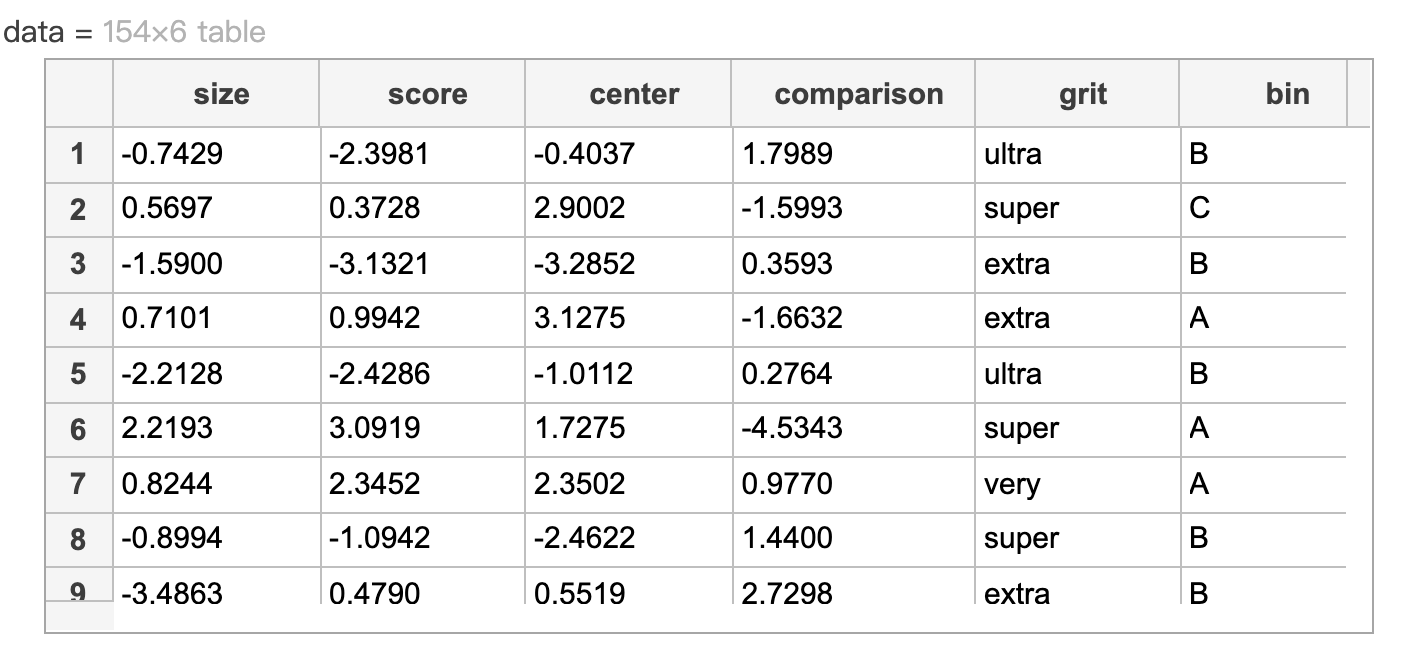
Create a numeric matrix of dummy predictors for the categorical data in 'data.grit'. Save it as 'dvGrit'.

dvGrit = dummyvar(data.grit)

Create a matrix named 'predictors' containing the numeric predictors in 'data' followed by the dummy predictors 'dvGrit'.

Use sequential feature selection with a kNN model to determine which variables to keep in the model. Name the logical vector 'toKeep'.

predictors = [data{:,1:4} dvGrit];

ferror = @(XTrain,yTrain,XTest,yTest)...

 nnz(yTest ~= predict(fitcknn(XTrain,yTrain),XTest));

toKeep = sequentialfs(ferror,predictors,data.bin)

Create a seven-fold cross-validated kNN model named 'mdlPart' with only the selected predictors. Calculate the loss with this model and name the result 'partLoss'.

mdlPart = fitcknn(predictors(:,toKeep),data.bin,"KFold",7);

partLoss = kfoldLoss(mdlPart)

範例

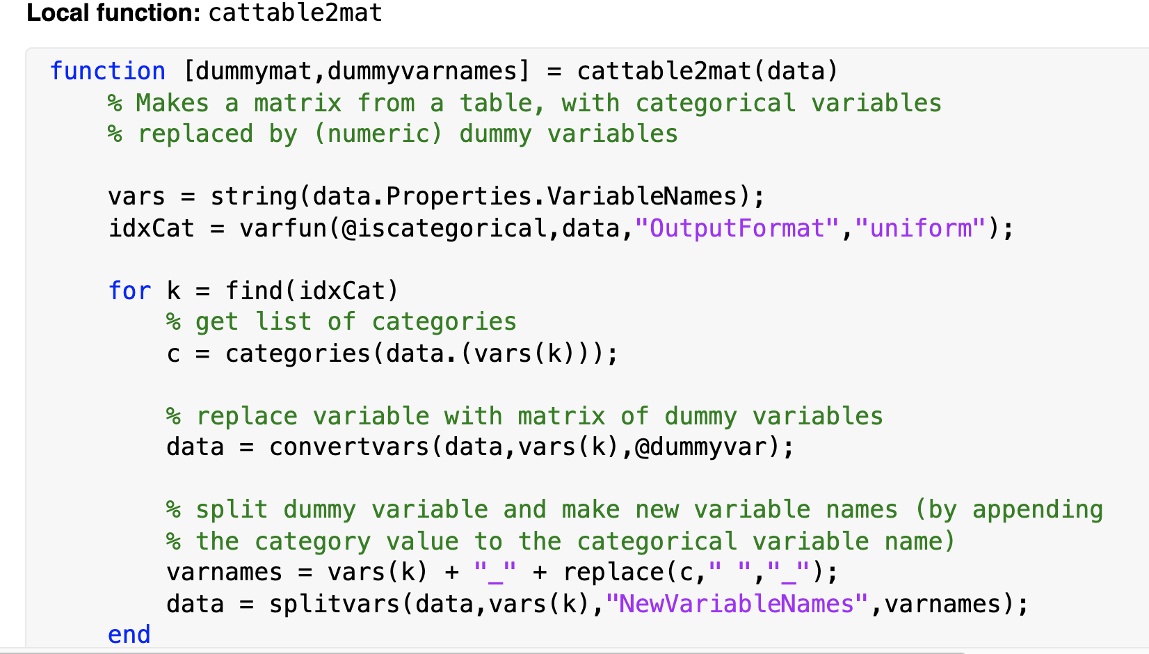
The open live script performs feature selection on a Naive Bayes classifier for the heart disease data set. You can look at the local function cattable2mat to see how dummy variables are created.

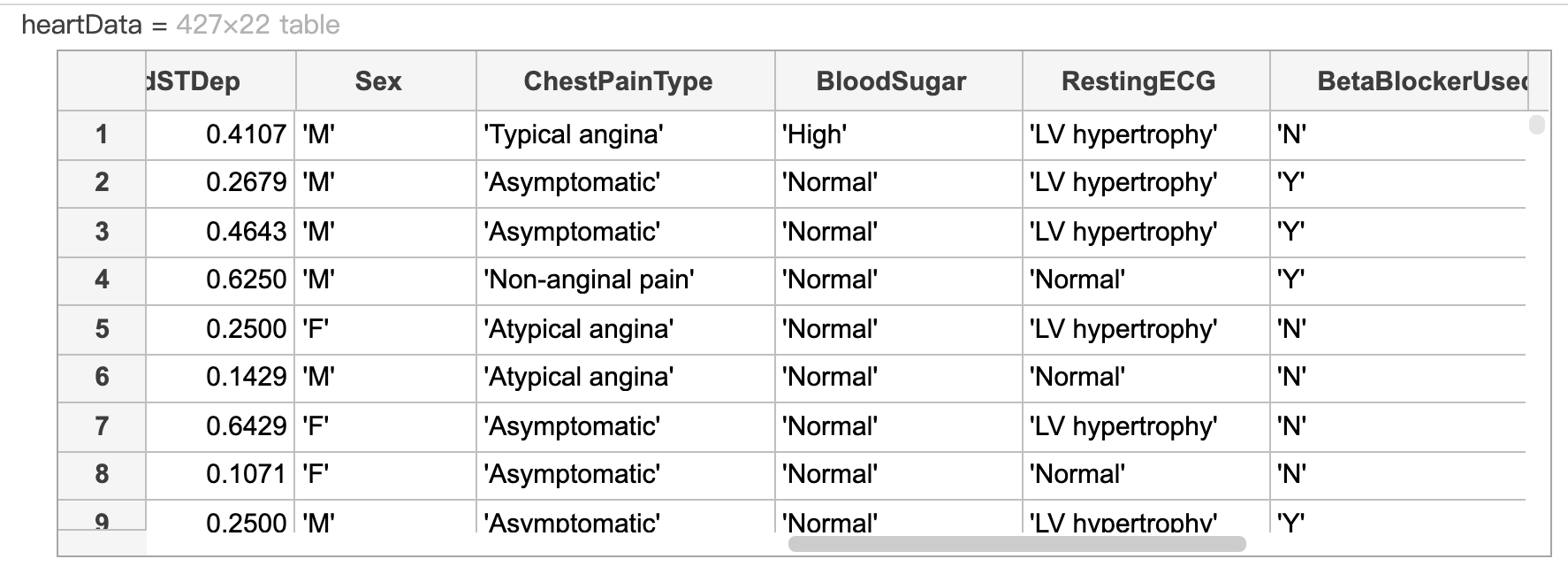
heartData = readtable("heartDataAll.txt");

heartData = convertvars(heartData,12:22,"categorical");

Extract the response variable and make a partition for evaluation.

HD = heartData.HeartDisease;

rng(1234)

cvpt = cvpartition(HD,"KFold",10);

Convert categorical predictors to numeric dummy variables

[X,XNames] = cattable2mat(heartData(:,1:end-1))

Fit a Naive Bayes model to the full data

dists = [repmat("kernel",1,11),repmat("mvmn",1,10)];

mFull = fitcnb(heartData,"HeartDisease",...

"DistributionNames",dists,"CVPartition",cvpt);

Perform sequential feature selection

rng(1234)

fmodel = @(X,y) fitcnb(X,y,"DistributionNames","kernel");

ferror = @(Xtrain,ytrain,Xtest,ytest)...

 nnz(predict(fmodel(Xtrain,ytrain),Xtest) ~= ytest);

toKeep = sequentialfs(ferror,X,HD,"cv",cvpt,"options",statset("Display","iter"));

% Which variables are in the final model?

XNames(toKeep)

% Fit a model with just the given variables

% Display loss values

lossFull = kfoldLoss(mFull)lossPart = kfoldLoss(mPart)